Almost exactly 3 years ago, I was in Salt Lake City for my first ever Cosyne. Right around that time, Nature Neuroscience had published a special issue on neural computation and theory, putting together a collection of reviews and perspectives outlining the importance of various theoretical and analytical advances for neuroscience, in light of our ability to collect more data and manipulate circuits more precisely. The Springer folks at Cosyne had a stack of it they were giving out for free, so obviously I picked one up. Over the next 3 years, this one magazine floated around my house - from my desk to the book shelf to the coffee table, even surviving a move, and eventually ending up as candidate bathroom reader. It was only after I got back from this Cosyne a few days ago that, for whatever reason, it occurred to me to read it. The opening piece was an overview by Anne Churchland and Larry Abbott, in which they go on to say:
Specifically, it is not clear how to reduce large and complex data sets into forms that are understandable. Simply averaging responses of many neurons could obscure important signals: neural populations often have massive diversity in cell type, projection target and response property. One solution to this problem is to leverage methods that are naturally suited to multi-neuron measurements. Correlations across neurons, for example, can offer insight into the connectivity and state of a network. Another solution to this problem is the use of machine-learning-based readouts and classifiers to interpret activity at the population level and relate it to behavior. […] In a study involving large-scale imaging of the C. elegans nervous system, a principal component–based description of neural activity was extracted, and patterns of activity across the entire neuronal population were correlated with behavioral states of the worm.
I chuckled to myself as I finished reading this 2-page commentary: had I read it when I picked it up 3 years ago, maybe I would’ve hard-pivoted and gotten on the #MANIFOLD train early, instead of screwing around with all this LFP and oscillation nonsense, because it is exactly this population latent factors type of work that has taken over Cosyne19. Funny enough, they also noted the rise of Yamins & DiCarlo “brain as deep convolutional neural network” type of work that took over CCN last year. It was neat to see Churchland & Abbott make this spot-on prediction, though in hindsight, it’s not exactly fortune-telling that two giants in the field predicted and/or influenced the direction computational neuroscience eventually moved towards. What’s more is that it made me realize that I’ve been around for long enough to see scientific trends shift, even though I often feel like a little fish swimming along, but squarely outside of this current.
Below are my notes from Cosyne19 in Lisbon/Cascais. I’ve organized the talks & posters I found interesting into a few broad themes (instead of chronologically), along with some synthesizing commentary of my own when I had them. As the intro suggests, a large part of it will center on latent factors/dynamics of neural populations types of work, just because those dominated the conference itself. Relatedly, a lot of presentations were on (data-drive) latent decomposition of behavior (behavior #MANIFOLD?), which I think are neat and potentially more impactful than neural manifolds in terms of understanding cognition. In addition to those, I highlight a set of works on the brain of a contextually embedded and embodied agent, and some deeper philosophical considerations. Finally, I end on some thoughts about attending Cosyne by myself and other general topics. Keep in mind that my understanding of these works are mostly based on intuition, especially geometric intuition, and some Google searches for things I had never heard of. So I apologize if I missed the point on any of them.
I realize this is less like a targeted blog post than me white-boarding out all my notes, and has gotten unapologetically long. Unless you’re procrastinating HARD on a Friday (which is totally valid), I recommend jumping to the sections of interest directly, though they do build off of each other:
- Neural #MANIFOLD:
- Latent factors, latent dynamics, stochastic nonlinear dynamical systems - and what next?
- Latent Dynamics of Behavior:
- Cognition is latent basis set of behavior?
- Context, Coding, & Causality:
- Embodied and embedded brain, and whether neurons “code”.
- General Conference & Other Random Thoughts:
- Go here for a (much) lighter reading.
Neural MANIFOLD
First, a (very) brief primer on latent variable/neural state space analysis: as the Churchland & Abbott article mentions above, we are now able to record hundreds to thousands of neurons simultaneously with probes like Neuropixel, and classical single-neuron techniques that average over neurons, stimulus, or trials (receptive field, peri-stimulus time histogram, etc.) lose a lot of interesting information. Historically, you’d more or less find neurons that respond to task during surgery and then record their response “for real” during the experiment. But when you record hundreds of neurons in an unbiased way (which is definitely the right way), it turns out that more often than not, single units do not show any stimulus specificity when their activity is averaged.
This is where Principal Component Analysis (PCA) and all its cousins comes in. Evidently, the firing rates of neurons are highly correlated. This is true during task, but also after accounting for task variables and during spontaneous behavior, the latter cases being unfortunately coined as “noise correlation”. All the latent factor/dynamics models, in essence, attempts to distill underlying structure from these pairwise neuronal correlations. In other words, we assume that there is some underlying driving variables that are causing many pairs of neurons to fire in a correlated manner. These are called “latent factors” because, well, they are sort of hidden/unobserved variables. Moreover, a slew of studies have recently found that these latent factors are low-dimensional, in that a few latent variables explain most of the variance in the original neural data, and that they correlate much better with task variables. Finally, “neural manifold” refers to the theoretical smooth “surface” or subspace, from which these latent variables are sampled from. I know there are still a lot of unexplained jargon above, and you can probably write a whole textbook on these methods and the underlying math. I want to do a full-blog post that link these concepts together soon, because, as we will later see, they are much more generally applicable than just on neural data. For now, this blurb should get you up to speed to digest the next set of talks, and my go-to dimensionality reduction reading is always this beautiful blog post by Alex Williams, and the Udell paper it links to.

For me, 3 of the invited talks really capture the 3 distinct flavors of latent variable analysis that were at Cosyne: latent factors (Ken Harris), latent dynamics (Sara Solla), and latent distributions (Maneesh Sahani). The first is closest to vanilla factor analysis (low-rank matrix decomposition), in that it simply accounts for the correlation structure within the data. The second adds an additional dimension of time, in that adjacent data points are temporally linked. The difference between these two is that you can shuffle the order of the data points in the first and retrieve the exact same result, whereas time obviously does not work that way. The last one adds yet another layer of complexity, which is stochasticity in the form of sampling from probability distributions, usually as a result of a nonlinear stochastic dynamical system. Keep in mind that these are my arbitrarily drawn boundaries, very much open for reinterpretation. (Figure from Saxena & Cunningham, 2019)
Latent Factors
Ken Harris presented results from Stringer et al., 2018 looking at the static latent response/code of 10,000 neurons in mouse V1 (it’s over 9,000!), measured via calcium imaging, while the animal views 2,800 naturalistic images. They use an in-house variant of PCA called cross-validated PCA, which looks for the shared correlation structure induced only by the image stimuli over two repeats, since spontaneous activity also introduces correlations, but is “non-coding”. The methods are in the preprint, so refer to that for details (it’s a good read). A lot of previous works have shown that task-induced neuronal correlation is often low-dimensional (a few large eigenvalues). Peiran Gao (Ganguli group, no relation) has a nice theory paper hypothesizing that that’s caused by the low-dimensionality of tasks. But in this case, naturalistic images should not be low-dimensional because there is information at every scale - from overall intensity, to blobs of objects, to fine-grained texture details.
Lo and behold, they found that the latent coding manifold in V1 is “appropriately” dimensional: not too low and not too high, straddling some Goldilock zone, as evidenced by the fact that the eigenvalues fall off via a decaying power law with an exponent slightly less than -1. In other words, each subsequent latent factor explains a fraction of the variance compared to the previous. Why is this fascinating? Ken Harris argues that the latent neural code has to balance orthogonality and smoothness. Orthogonality is analogous to information density of the latent factors, where a flat eigenspectrum (equal eigenvalues) means each latent factor accounts for the same amount of variance in the data. Smoothness is in reference to the latent manifold, and it’s a nice property to have because, presumably, the code has to be continuous (and differentiable?). If the eigenvalues don’t decay fast enough, that implies the code is dominated by high-frequency content when integrated over all dimensions (though I’m not sure if there’s some natural ordering of the eigenvalues other than magnitude, like in Fourier decomposition). If they fall off too fast, then most of the variance is in the first few dimensions, making it a redundant code. They do some nice control experiments to show that the exponent of the eigenspectrum decay tracks, not image statistics, but image dimensionality. He goes on to talk about holographic coding and the infinite-neuron cortex, because why not.
A few other talks I liked along this vein: for example, Alex Cayco Gajic presented calcium imaging data from parallel fibers (axons) of granule cells in the mouse cerebellum, and showed that there is also low-dimensional structure there after PCA. Similarly, Andrew Leifer gave a talked titled “Predicting natural behavior from brain-wide neural activity”. I gotta say, this was hella clickbait, because I was expecting at least mice and got very excited. But it was in C. elegans. That being said, it was a great talk. They use PCA to find latent structure in all the neurons in the worm brain to predict behavioral measures like velocity and heading angle, and they also generated fake videos of worms locomoting from the brain activity.
As an aside, the Ken Harris talk was one of my favorites, because it links neural population coding to something I hold close to my heart: 1/f power law decay in time/frequency. I almost did a spit-take when he said the words “1/f power spectrum” and “fractals” in front of 500 people at Cosyne. Am I fucking dreaming? Those are edgy words even in the LFP world, and all of a sudden they’re cool in systems comp neuro? If you’re a regular reader of this blog and the VoytekLab, you will know that the power spectrum of neural time series (EEG, LFP, etc.) also has a 1/f decay. The two concepts are exactly analogous, the difference being that the former describes “space” with a data-driven basis set (principal components), while the latter, Fourier spectrum, describes time with a predefined orthogonal basis set that is the complex sinusoids.

1/f power spectrum in the rat hippocampus.
In fact, my only “complaint” is that this work doesn’t address the temporal component at all, because the measured neural activity are static and kinda averaged over all time points in the trial (or represent the end points), limited by the slow dynamics of GCaMP. But how the population traverses through this trajectory from one point to the next and reaching the stationary points for coding is really important, because you’d hope similar images are closer together in the neural manifold, lest the neurons have to bounce all over the place from one frame to another during a movie or something. Interestingly, a poster by O.J. Henaff & Y. Bai (Goris & Simoncelli group) actually addresses this point in monkey V1. They hypothesize that the visual system transforms temporally-continous inputs (i.e., natural videos) such that it minimizes the curvature of the latent neural trajectory when driven by such inputs, which they term “neural straightening”. They previously show evidence of this in human behavior with a really nice task (to come out in Nature Neuro, I believe). This poster presents some new data showing that neural population dynamics in monkey V1 also experiences this straightening. See here for a general computational model (sparse manifold transform) that is consistent with these types of data.
In any case, I’ve become very interested in the translation between space and time in the last few months (e.g., ergodicity), so if you have any thoughts on this, please slide into my Twitter DM.
Latent Trajectories
Speaking of time, Sara Solla presented some biorxived work by Juan Álvaro Gallego et al. looking at the consistency of movement representation in neurodynamics, i.e. its temporal trajectory in phase space. Juan’s tweet thread is a great primer on the work. I really liked her framing of the problem from an engineering/practical perspective: the particular neurons we record in an experiment varies over months, which means the “population” firing response will be different to the same stimulus/motor command on different days, so how can we construct decoders that will translate between neural activity to motor action (e.g., for BCI) that will be stable over a long period of time? If you get a neuroprosthetic implant, you don’t want to wake up and spend half an hour training the damn algorithm every single day because the probe moved half a millimeter when you were tossing around in bed at night.
The theoretical machinery they use is, again, the latent neural manifold/subspace. The assumption is that the M1 subpopulation, as a whole, encodes the representation of the same arm movement as the same path on the same manifold, and the recorded neural activity is just that identical manifold projected onto different “neuron axes”, which are randomly sampled by the probes each day. Therefore, in theory, the latent subspace you recover from day 1 and day 800 should be the same, assuming you’ve sampled enough neurons to at least recover the full manifold. So if you do PCA on the [neuron x time] matrix of each trial, you should recover PCs that represent trajectory traversing the manifold, from task onset to end, that is the neural representation of a continuous arm movement. If you compare these trajectories on different days, they should be identical (or very similar) for the same movement, which is precisely what they found.

There’s a caveat here, which is that the manifold PCA recovers is subject to rotation on different days, because the principal components are constrained to be linear combinations of the sampled activity, so you can retrieve the axes of the original manifold, but only relative to each other, not in absolute. Let’s say you turn some crank and the same football falls out, but it lands differently (i.e., is rotated) on different days. How do we undo this rotation if you want to compare the different balls? You just have to take one of the footballs as the relative reference, and rotate all the other ones you get to match it as closely as possible, and then evaluate how similar they are. In math, this whole operation is called canonical correlation analysis (CCA), which is a pair of PCAs and then a rotation.
So after 172386 singular value decompositions, you get a set of aligned principal components for each day of the experiment, and they find that the retrieved trajectories are remarkably similar over more than 2 years in the same monkey doing the same task, measured both as similarity and decoding accuracy. In other words, like your mailman traveling the same path day after day, it’s only our perspective that has changed, and us sampling different neurons is like standing on a different hill while we watch the mailman walk seemingly different paths. This is a remarkable result, because it goes beyond showing that the latent manifold is low-dimensional, it also implies a stable manifold over time, presumably representing the learned task structure. I’m very curious to see how the manifold changes in the early days of learning the task, though. Does it follow some kind of optimization/efficient coding algorithm, similar to the neural-straightening hypothesis above for visual perception?
Non-linear Stochastic Dynamical Systems
You will notice that even though the work above deals with trajectories in time, the methods they use for finding the latent dynamics are agnostic to time. Meaning, if you shuffle the time indices of each recording in the same way, the results will be identical, though the plots won’t be as pretty/interpretable. Furthermore, it does not explicitly deal with noise in a probabilistic sense, it’s just another source of variance to remove. These aren’t necessarily limitations, since, if the experimental design allows it, it’s probably better to use the simplest method possible, which, in this case, is matrix factorization/reconstruction under Gaussian errors. To describe brain dynamics in its full glory, we can model it as a nonlinear stochastic dynamical system, which was the third broad flavor of neural #manifold at Cosyne. Maneesh Sahani gave a keynote on Distributed (or Doubly) Distributional Codes(DDC), which, I gotta admit, lost me after 5 minutes. I did, I think, understand the premise of issue, which is that uncertainty in the world seems to be explicitly accounted for by us, at least behaviorally. So a deterministic model of the brain that does not represent distributions will suffer in performance compared to an optimal agent, especially with limited information/training samples. I won’t attempt to butcher this farther, just pointing you to the relevant resources here and here instead. My favorite out-of-context quote of the conference was during this talk, though, when he says:
“I seem to have lost my joint.”
A related work I liked a lot is a poster presentation by his colleague (trainee?), Lea Duncker, who talked about using Gaussian Processes to model continuous-time latent stochastic dynamical systems. I struggled with the preprint when it came out, so it was really helpful to hear her explain it in person. Even so, I really have to read it again to retell it with any confidence, so instead of subjecting you to that, I will just say why I like it and think it’s important:
Conceptually, a “dynamical system” is just a flow field, defined by some function f(x) such that at every point x, f(x) tells you where you should go towards next. So given a starting point (initial condition), you only have to consult this flow function at every infinitismal time step along the way and deterministically live out your life. This can model fluids, charged particles, abstract quantities like population in an ecosystem, or in our case, the “flow” of a population of neurons firing. A lot of the latent factors methods, like PCA, can retrieve trajectories on the empirical subspace spanned by the observed data, but cannot make generalizations about the hypothesized dynamical system as a whole or describe it. What we really want is a method to learn the flow map (or phase portrait) of the entire field/manifold, such that given a hypothetical starting point we’ve never seen, we can know where we will end up. The appeal of these kinds of methods is that it goes way beyond just neuroscience. If you can define a set of variables, abstract or physical, and how they should change over time via some differential equations, then such a method can theoretically retrieve it. In the context of neuroscience, this will give you predictions on how a novel stimulus may drive population activity. Her work doesn’t get us there all the way (that would be the holy grail, I think), but it’s a step towards it. In particular, with Gaussian Processes, uncertainty of the dynamics is reduced (clamped) at where you have observations, and flow on the rest of the field can be inferred with some bound on uncertainty. Similarly, Daniel Hernandez presented his work on Variational Inference for Nonlinear Dynamics, which tries to solve the same general problem as well. The main difference here is that instead of modeling a continuous-time flow field, VIND approximates transition probabilities at discrete time points using Gaussians (this is the variational inference part).
A digression for a funny story here: Daniel’s poster was in the same session as me, so I only happened upon it when I was doing a quick walkthrough at 12am, after the session officially ended. His poster looked really interesting, so I stared at it for a while, hoping that I could get a gist just from reading (I couldn’t). He saw me, and my guy had enough energy at midnight to offer me a full rundown, which I just could not say no to. 1 minute into it, I told him: “man, this is really cool work, but I just stood at my poster for 4 hours and I am not registering a single word you’re saying to me right now. So I’m gonna take a picture of your poster and go check out your preprint.” He had a hearty laughed, told me he liked my tattoo, and then gave me a big ol’ hug. Probably the most pleasant and human interaction I’ve had at a poster ever, and because of this, I am committed to go through his paper in its full mathematical glory.
Another talk along this line was by Daniel O’Shea, who developed and used “LFADS 2.0” to learn the latent dynamics of brain-wide population response (in mouse this time!!). Using neuropixel probes, they recorded a gajillion neurons across many brain areas but over many days, which presented the same problem as what Sara Solla talked about, namely, separately-recorded neurons contributing to the same task. Similar to all the other approaches above, the original LFADS (Latent Factor Analysis via Dynamical System) learns the (nonlinear) latent dynamics, but takes what I call the “fuck it” route and uses a recurrent neural network to approximate the trajectories through the latent neural manifold. The recorded neural population response, then, is assumed to be the result of some linear (readout) projection of that trajectory, then a nonlinearity and a Poisson stage. Most importantly, it does this at the single trial level, which is very nice because trial-to-trial variability is not just measurement noise, but brain response as well. (I put it in this section because of the variational autoencoder, though it doesn’t learn explicit probability distributions in the same sense as DDC). In LFADS 2.0, the separately recorded populations are still assumed to contribute to the same underlying manifold, but instead of aligning them through rotation like above, it basically assumes and learns a different readout stage for each day. Pretty neat idea. Check out Daniel’s tweet thread for a great explanation and some mesmerizing gifs.
Beyond the Neural Manifold?
All of the above latent space works are cool in their own ways, using different mathematical machinery to tackle the same problem, and applying them in different neural systems doing different tasks. But having followed this line of work for a while as an outsider, and after seeing so many of these talks in rapid succession, one question nags me: what are the actual state variables in the retrieved latent manifolds? To be more specific, in a dynamical systems model of some natural phenomenon, the state variables usually represent something concrete. You can’t always directly measure them, and they’re not always physical quantities, but you assume they are what defines your flow field in the generative process. For example, the Hodgkin-Huxley neuron is a dynamical systems model of action potential generation, where the 4 state variables are voltage and 3 channel (in)activation variables for sodium and potassium.

In the neural population state space formulation, I rarely see any works exploring just what x is in f(x)? Obviously there isn’t some magic manifold box in the brain that generates the latent dynamics and then projects them onto brain cells, so what are the empirical dimensions of this latent space actually representing? My intuition says that they are, of course, some other neural variable. Maybe the space is spanned by the amount of dopamine, acetylcholine, and serotonin in the local area. Or maybe it’s a coupling of heart rate and breath rate. More relevant for cortical computation, though, it probably represents the correlated firing of the afferent (input) area, e.g., the manifold in V2 represents some correlated inputs from V1. Joao Semedo touches on this in his talk during one of the workshop sessions. In that work, he finds that single-unit activity in V2 can be predicted by activity from about 2 V1 cells using a low-rank linear regression, just as well as you can with all the V1 cells. In other words, activity of each V2 cell is spanned by just 2 dimensions in the subspace of V1 cells. In contrast, an efferent region in V1 required more dimensions to reconstruct, so fluctuations in V1 can be used sparsely to predict V2 activity, but not V1 activity. Most interestingly, dimensions of the intrinsic V1 manifold that explain the most variance (through factor analysis again) do not predict V2 cell activity as well. I think this makes sense in the input-output framework: the principal components of V1 subspace may correspond better to single-unit firing of its input area (i.e., LGN), which V1 transforms and projects to V2. Here, they predict V2 firing directly, and I wonder how well V2’s PCs can be predicted by V1 activity, as well as V1’s PCs.
Reaching a similar point from a different perspective, Scott Linderman gave a talk on constraining statistical and dynamical models of neural data using computational theories. I think it’s related to this paper, but with much more emphasis on the latent factors types of model. He had a sick slide with this table cataloging all the latent factors models people use. The point, I think, remains the same: while a data-driven approach can uncover, for example, sophisticated empirical subspaces, to reach some kind of “understanding”, we have to integrate it with (computational) theories, be that a cognitive computation or a neural computation, more or less of the box and arrow variety. More specifically, using factor analysis, we find that neural populations are low-dimensional (massively correlated) and traverse conserved trajectories (stable), how do we advance our understanding of the brain? What would that understanding even look like?
Latent Dynamics of Behavior
Putting cognition aside, “understanding” in systems neuroscience probably means relating neural activity to sensorimotor transformations required for the organism, as an embodied agent, to implement adaptive and efficient behaviors. No matter what school of thought you come from, the brain is the middle stage between all sensory inputs and all motor outputs (spinal reflexes notwithstanding). To understand brain and behavior, though, you have to have a good idea of what behavior is as well, because it’s certainly not sitting in front of a computer monitor pressing keys a thousand times in response to visual stimuli. That’s why I was glad to see a lot of work at this Cosyne on characterizing and decomposing naturalistic behavior, especially in the “Quantifying social behavior” workshop, using similar mathematical machinery as the ones above for neural data. At the end of the day, these are all just multidimensional tensors or time series, so it’s pretty natural to apply across domains, with the same goal of finding a dimensionality-reduced representation of the data.
In the case of behavior, dimensionality reduction usually means quantifying position, motion, or joint angle vectors from video, which are then submitted for further analysis and modeling. To do that, animal (or human) subjects usually have to wear some kind of reflective marker that indicates where the physical features of interest are (I always think of this goofy video), or have undergrads hand label millions of video frames if a more abstract gesture can be directly inferred. Both of those are unideal for obvious reasons. Blowing all that to prehistoric times, Mackenzie Mathis talked about DeepLabCut (paper), which uses a DEEP artificial neural network (ResNet) initialized with weights as trained on ImageNet (a fuck-ton of images), to track animal body parts without reflective markers. You have to give it a handful of hand-labeled images to optimize it, but it seems to learn rather quickly. This is one of those things that you just want to throw everything at to see what you can get out, especially for human behavior. Gone are the days of setting up XBox motion tracking in the lab (maybe)! In the same workshop, someone talked about using DeepLabCut to track mouse mating behavior. I didn’t catch his name and it was during John Cunningham’s slot, so I assume it’s someone in his lab. Specifically, by tracking two mice’s positions over time, they were able to use the change in their relative movements during pursuit to quantify a development of their relationship over longer timescales. Finally, I saw Adam Calhoun give a talk about his work on quantifying fly courtship behavior, using Hidden Markov Model and GLM to model the transition between latent behavioral states, finding some rather unexpected and unintuitive states, like a male fly just chilling during the “doing whatever” state (lol).
From all this, I gather that systems neuroscience might be converging onto one huge canonical correlation analysis: on the one end, you can measure latent behavioral states that describes observable behaviors compactly. On the other end, you can measure latent neural states that describes measured brain dynamics compactly. The natural next step is to see if these low-dimensional representations are better correlated and more effectively manipulated than behavior and neurodynamics in their original spaces. So far, we’ve seen works that relate monkey arm velocity (native behavior space) to the latent neural space in M1, and Adam touched on manipulating behavioral latents with optogenetic stimulation of a neural circuit (native neural space). Note that in both cases, the dimensionality reduction was done manually by the experimenter, as the result of a specific intention to isolate variables of interest. It’d be quite straightforward to combine the two approaches and compare one latent space to another without squashing variability a priori, because, well, humans have experimental biases. This is a pretty exciting direction, I think, and will probably start showing up at Cosyne in the next year or two. Definitely looking forward to that one.
What I also really want to know is this: humans infer intentions of other humans based on a set of prior assumptions updated by immediate observations of their physical gestures, be it facial, bodily, or whatever. In some sense, I think cognition (and cognitive processes) are the latent dimensions of human behavior learned by our brains. These have served us well as human beings for centuries, especially with the help of language to fine-tune any rough edges during social interactions. However, they might not serve us as well as scientists, since cognitive (neuro)science and psychology often take these latents, sometimes now referred to as folk psychological constructs, and study them as if they’re objective and quantifiable things. So what I want to know is how well empirical latents measured through physical behavior match our learned latents as humans, and where do they differ. I have no doubt that folk psychological constructs - things like emotion, intention, attention, etc - can capture a large amount of variance in physical behavior. That’s probably why they still exist. But maybe those only partially overlap the “true” or objective latents. I guess I’m asking for a quick-start manual for understanding human behavior during social interactions for the socially awkward (hello hi). What’s even more confusing, though, is that behavioral latents must account for contextual information, because the same behavior may mean very different things in different physical and social environments.
Context, Coding, and Causality
We’re really in the deep end now, ladies and gentlemen. Computational and systems neuroscience doesn’t really have a good track record as far as taking into consideration embodied and embedded cognition. Part of this is due to the early success of input-output models of early sensory processing, part of this is probably due to the fact that it’s easier to run experiments that control for and constrain environmental variables. I’m not throwing shade on the field - there’s a now infamous story of me saying something completely stupid during my first day of grad school in Cognitive Science along those lines. My point is just that it’s rather surprising to see a discussion of environmental context, embodied cognition, and circular causality at Cosyne, of all conferences. These were probably some of my favorite talks since they border on philosophical, but also link in a lot of ideas that are new to me.
Embedded and Embodied Cognition
Kim Stachenfeld talked about updated work on learning goal-drive structured representations of space in the hippocampal-entorhinal system, but from the perspective of training a reinforcement learning agent. The hippocampus was thought to sparsely encode/represent space via place cells for a very long time, but recent work has shown that it’s also able to represent more abstract “locations”, and in a goal-driven manner. From the perspective of a learning agent, you want to represent the most important aspects of space, so a natural question to ask is: what is a low-dimensional representation of space that can capture the most important aspects? One option is to just take a 2D Fourier transform of space and retrieve modes sorted by their eigenvalues, much like a temporal FT. The issue is, that assumes space is homogeneous, which is not true because 1) there are often physical boundaries in actual space, and 2) there are abstract structures with respect to some goal that can serve as useful boundaries of space, even though they are “imaginary”. One example she gave was that when a rat is placed at the bottom of a V-shaped maze, and it knows that there is a reward at the end of one of the arms, it’s not efficient to represent each arm as a series of many homogeneous steps that lead you to the end. Instead, you really just care about which of the two arms will be rewarding, and to book it to the endpoint where the reward is.

So instead of a naive Fourier transform, she proposes using features derived from factorizing the graph Laplacian matrix, or Laplacian eigenmap. Briefly, the Laplacian matrix describes the degree and connectivity of nodes in a graph, which, in the above case, are discretized locations in space. So this is like the graph-equivalent of a correlation matrix, taking into consideration heterogeneity of connectivity, which you can then decompose using your favorite matrix factorization tool to retrieve the latent dimensions/basis. The main takeaway here is that 1) entorhinal cortex grid cells might learn something like such a structured basis set which the hippocampus uses to construct place representations, and 2) these structured features, when given to an artificial RL agent, enable them to learn tasks much better. One of the improvements is that agents can now “explore” more efficiently, in a non-homogeneous way, which is referred to as Levy walk/flight or super-diffusion, instead of meandering around via Brownian random walk. Put it differently, the agent can now explore at different spatial scales, whereas Brownian motion is restricted to movements at the same scale (defined by the normal distribution of the steps). There’s some evidence that real foraging animals explore space in exactly this way, which is really, really cool.
I liked this work a lot because it looks for structures in a complex environment, instead looking just at neural dynamics in a reduced environment. I also learned a ton from this talk, but I think the biggest mindfuck was thinking of the hippocampal system as doing eigendecomposition on structured space. Neurons in V1 are selective to spatial frequency, while the cochlea almost literally performs Fourier transforms on sound. But to think that the hippocampal system does something similar as well was just too much for me to handle. In some sense, that’s not too surprising, since the idea that the brain looks for structures in the world is not new, and that some of our eigen-decomposition algorithms just so happens to approximate what the brain does. On top of that, many of the early neuroscience experiments were done in the spirit of linear systems characterization, i.e. input-output transformations, where the system is characterized by its linear response function (to sinusoids). I’m sure that as we invent more sophisticated decomposition techniques, we will strap them onto analogous transforms that the brain is doing. That being said, I definitely had a moment during the talk where I was like:
“holy smokes the BRAIN IS ONE BIG FOURIER TRANSFORM?”
Two other talks I found fascinating: first, Tom Hindmarsh Sten talked about a really serendipitous finding where, during reinforcement learning tasks, mice show much faster acquisition of task knowledge if you include “probe” trials where the cues are still presented but the rewards are removed (see tweet thread). It’s literally the exact same task, the only thing that’s different is whether the juice dropper is there or not. If you just measure task performance on reinforced trials, the animals seem to learn much slower, and with greater variability in learning time. This is so relatable it hurts - you study all week for an exam, and you can do the practice questions with your eyes closed, but for whatever reason, during the exam itself, your brain just freezes on even the easiest questions. But more seriously, this gets at a really interesting question about experimental design: how do we know that the behavioral and neural variable of interest - in this case, simple task knowledge - is actually measured by the task we employ? Like the exam example above demonstrates, our cognition is flexible and dynamic, even in something as simple as a conditioned response. Or maybe on some trials the mice just don’t want to drink juice. Who the hell knows? Well, certainly not neuroscientists if we keep using just one task to probe a single cognitive phenomenon of interest. This work doesn’t just test context-mediated behavior, it reveals a blind spot in behavioral experiments, and really advocates for accounting for a broad set of behavioral and environmental variables. Also, I thought it was cool that this provides some insight as to why unstructured play/exploration is important for children in learning generalizable rules, and probably adults too.
In another neat talk, Grigori Guitchounts presented data on mouse V1 neurons “encoding” roll, pitch, and yaw (rotational vectors) of the animals head, to a point that the rotational vectors can be decoded using V1 firing. Additionally, they show that M2 lesion disrupts that “encoding”. “Encoding” is purposefully enclosed in scare-quotes here. If you ask any self-respecting neuroscientist what V1 neurons do, they’d tell you that they encode low-level visual features. That is, after all, the “computation” V1 neurons perform. Does this piece of data contradict that? Well, something something feedback projections. Plus, the brain has to account for self-motion somewhere when it processes the visual scene, otherwise it’d be shaking all the time. But wait, why is it that when V1 neurons fire to visual stimuli, they are “encoding” visual features, but we’d be hesitant to say they “encode” movement variables?
Do Neurons Code?
I did my best to not get into that “coding” debate on Twitter, but Romain Brett gave a talk on his BBS paper in the Causality workshop, and I have to say I absolutely loved it. I get weirdly bothered when people say neurons “encode” information, so whenever I get into this conversation with somebody, I say something like, “well, does a rock encode its velocity as it tumbles down a cliff?”. That inevitably elicits some staring, and shrugs, like “okay there buddy”. His talk (obviously) is a much more sophisticated treatment of that argument. He argues that “coding” only occurs from the perspective of the neuroscience experiment, as a response to a particular stimulus the experimenter is interested in, but may be completely meaningless outside of the context of that particular experiment. The example he gave was the Jennifer Aniston neuron: let’s say you flash an image of Jennifer Aniston, and some neuron reliably respond to it, you might say that that neuron encodes for Jennifer Aniston, but what if it fires when the image is absent? What does that Jennifer Aniston neuron do when you’re out and about in the world not looking at Jennifer 99.9% of the time? Does it just do nothing? Yes, the grandmother cell example is ridiculous, but the same thing applies to any concept - what do orientation-tuned neurons do when you’re not looking at gratings? Or when you close your eyes?
…
So I just ended up writing a whole essay, and this is not the first of such essays I’ve stream-of-consciousnessed on this exact thing. In the interest of time and space, I’ve removed it. People that care about this kind of thing, just go read the paper, and I’d love to have a discussion on this topic (but not on Twitter for the love of god). I will just give you my own take here: I think the issue is not so much “coding” but “representation” (and maybe Romain uses those interchangeably, it’s been some time since I read it). What kind of things are we willing to allow for when we talk about neural representations? Most things are concepts entirely constructed by humans with an embedded social, cultural and linguistic context, and if you’re looking for that in the brain and arguing that the brain “encodes” it, like Jennifer Aniston or your Grandma, you’re probably standing on shaky ground. At the same time, the brain performs sensory-motor transformations with some history-dependence, modulated by various other systems in the body, so it certainly takes in, transforms, and sends out “signals”.
The key disconnect we, as experimenters, need to be aware of is that what those signals mean for us may very well mean different things for the brain, but we are stuck playing 20-questions with the brain while speaking completely different languages. For example, place cells respond reliably to isolated areas in 2D space, or so our interpretation goes. But why would a rat need a cell in the hippocampus to tell it where it is in an environment that has no relevance to it? Do we think the current space is always spanned by some set of cells in the hippocampus, and we just don’t have the density to record them all? Also, so what if the place cell fires? What downstream areas actually care? I think there’s some very implicit belief that spikes have an “end result” that triggers an outcome in “the mind”, i.e., the place cell tells the mind “I’m here!”. Whether that’s true is beyond me right now, but there are certainly downstream consequences to that cell firing. There almost has to be, otherwise it’s a huge energy waste. I think the pragmatic takeaway from this debate is that we should really focus on the communication and transformation of signals between brain regions, as many of the relevant ones as we can account for, instead of obsessing over what isolated regions are “encoding” for and testing them one at a time.
Interacting Systems and Circular Causality
Giuseppe Longo gave a tele-talk along similar veins on the differential method in biology, but coming from a more historical perspective, integrating various developments in mathematics, physics, and molecular biology. He argues that biology, and by extension, neuroscience, may fare better if we set out to characterize interactions, instead of causality. An example he gave was gravitation: we used to think of gravity as the planet exerting a force on other objects, until we realized that it’s really an interactive force that governs celestial dynamics as well as everyday objects around us, which opens up a fuller investigation of the physics. In biology, we tend to think of causal factors, like stimulus causing neural activity, which limits our thinking to a smaller set of variables. This is perhaps done by necessity, as biology has many more moving components, though perhaps we haven’t found the most efficient level of description. Either way, he argues for characterizing a much fuller set of system states and variables. In the context of neuroscience, that’s embedded and embodied. I’m pretty convinced at this point that one could have a very productive career in neuroscience just by following the works of Francisco Varela and Walter Freeman.
Finally, Ehud Ahissar caps off the Causality workshop by talking about active sensing and arguing that perception is a close-loop process, giving a range of experimental evidence from different sensory modalities. His conceptualization is one of circular causality, i.e., imagine a spiral that is circling around but also moving forward at the same time, where “real” time flows along the trajectory, while perceptual time flows directly through the longitudinal axis, since we are almost always imperceptive to the feedback that occurs to alter our perception at every time step. I really liked this talk as well, because how could the brain be set up any other way? All kinds of unexpected and strong sensory stimuli come in all the time, so either there is always a dampening mechanism at work to prevent us from having seizures all the time, or the brain is somehow designed to be perfectly calibrated at the right level of sensitivity to the wide range of things we experience. Actually, he makes a point to address this as well, and says that the sensory system can work in an open-loop fashion, but activity is always dynamic, and there is a transient response that settles into equilibrium. I think the point is that a transient sensory percept could actually be the product of a neural response at equilibrium.
Capping Off & Conference Thoughts
This has already gotten much longer than I’d intended it to be, but those were the huge amount of notes & thoughts I had because those works were genuinely all fascinating. Before signing off, just a few more things:
-
One last point about some science, actually: I had wanted to include the few oscillations/LFP works I saw there, but decided against it to keep a competitive advantage (kidding). Most notable ones include Terry Sejnowski’s talk on traveling waves in marmosets and babies, Tatiana Engel’s talk on global cortical fluctuations and its influence on perception, and Ethan Solomon’s poster on human hippocampal theta predicting semantic similarity during a free recall task. The first two have been published for some time now so just go read the papers. The reason why I call it competitive advantage (which I’m now giving away for free) is that these works point to an aspect of mesoscale population dynamics that I think the #manifold community will eventually converge on as well, but from the bottom up. More specifically, a low-dimensional subspace comes from massively structured (correlated) activity, and what’s a signal you can measure to get that for a nickel? Furthermore, they offer a new way of thinking about the cortex - as a medium - in which energy propagates in a wave-like fashion, creating all kinds of interesting spatiotemporal patterns. From this point of view, the connectivity of the cortical sheet plays a much bigger role in determining the dynamics, instead of some abstract latent variables that span the manifold to perform some “coding”. Terry actually went on to say: “that’s how the universe works.” So take it from him. Anyway, no need to belabor this point either, see the last blog post for the full rant. But I’d give it no more than 3 years until “the #manifold people suddenly all start talking about oscillations like they fucking discovered it”, to quote a friend. I fully intend on not missing that train, but in case I do, I will point to this paragraph as proof that at least I saw it coming.
-
I liked Weiji Ma’s tutorial on Bayesian modeling of behavior, and his follow-up points on model selection. The biggest reason for that, I think, is leaving time for people to work on the derivations and discuss with each other & the TAs. Even though I’ve gone through the math in various classes, I feel like I actually learned something because I had to work through setting up the problem, instead of just applying the formula to an already well-constructed exam question. Shout-out to his team of TAs! The other event I really liked, which I was super fortunate to get into, was the experimentalist+computationalist match-making session. It was great to just meet people and have extended conversations, and it was really motivating to hear about their experiments and what they’re interested in, for no other reason than that it’s interesting. Also, it was hilarious how a few experimentalist, upon hearing about my interest in the LFP, had offered spiking & LFP data on the side like it was hush money. It’s like this thing that people collect and toss in a change jar or the attic for later, but it also warms my heart to hear how many of them also had questions and interests in the LFP. This definitely contributed to me feeling validated.
-
Good to see the Cosyne committee taking on an active effort to increase diversity, especially representation of women. Clearly, comp neuro has a long way to go in terms of several aspects of diversity. I think I saw one - as in, a single - black dude at the whole conference. Obviously it’s not so much Cosyne’s fault than it is the field in general, which is something I’m not gonna get into here. Double-blind review is a great way of doing things, for sure, not just for gender balance, but also increasing the representation of smaller labs doing really interesting work. I’m sure the reviewers do their best to be objective, but somehow I have a feeling that “Surya Ganguli” or “Jonathan Pillow” carry more weight instinctively, than a lesser-known scientist. I’m not saying they or their students don’t deserve to be there, of course not. I love looking at their stuff too, that’s the point. People are always going to be interested in their work, but the conference should also be an opportunity to find people whose feed you don’t (but will) subscribe to.
-
On the conference experience overall: the first few days were pretty rough for me. While the talks were all very interesting and inspiring, none of it were particularly relevant for me. That by itself is fine, even good from my point of view, because it ultimately exposed me to works that I may not come across naturally. But because I was there all by myself, I had gotten it into my head that nobody cares about my work, and therefore have no interest in talking to me, which made it more isolating. Overall, I think going to a conference alone, especially in a foreign country, is tough, and it’s harder when you nor your advisor are well-known in that particular community. Furthermore, academics are already not the best at socializing, myself included, so having that extra barrier of working on totally different things makes it a little harder to establish any common ground. All this is to say that, if you find a straggler that looks like they’re just floating around at a conference, be kind and adopt them! I will certainly make an active effort to do so at the next conference, which is looking like CNS…tomorrow. In fact, if you’ve read this, please take it as an open invitation to say hi (if you want to). Nothing boosts my ego more than talking to people who has read my stuff, obviously.
-
That situation eventually got over itself. I decided “fuck it” and walked into a very local-looking restaurant where nobody spoke a word of English and got very nice fish for cheap. Then I met some kind folks from Berkeley that took me in and invited me to dinner and stuff, as well as connected with people who answered my lonely cry for food adventures on Twitter. Actually, the people I ended up hanging out the most with are those I’ve interacted with on Twitter to some capacity (and thank you all for not being strangers!) I gotta say, for all the time I waste on Twitter, it’s really a great tool to faciliate in-person interactions, even if all it allows for is a “hi I follow you on Twitter lol.” It’s just really fucking awkward to walk up to someone for literally no reason and try to strike up a conversation, conference or not, though I try to make a point to tell people that I’ve enjoyed their talks/posters, or I like their shirt or earrings or tattoo or whatever.
-
The Cosyne crowd is certainly on a different level: poster sessions run from 8pm to 12am officially, but people regularly stay till 1-1:30am. This is truly incredible and inspiring to see because it’s just a bunch of huge nerds getting into the nitty gritty of shit they really care about. I genuinely don’t know how people do it, at least not in a bar after several drinks. The other thing is - holy shit - they pack the poster hall like a can of Portugeuse sardine, which was true in SLC as well. Use large fonts and less words on the posters, along with the key takeaways, please. This just makes everyone’s life easier. It’s impossible to stay at every interesting poster to wait for the start of a go-around, so it just makes everything much more efficient if someone can follow along with the main points by reading, and come back later for clarifications if needed.
-
Most importantly, my all-time favorite conference quote:
“c’mon, the macarena can’t be harder than spectral analysis!”
So I’ve been bumping this non-stop for the last 6 months (#BABISH), only to find out that this is literally hotel lobby music. As in, I was in the bathroom and thought I’d somehow gotten my music to play from the hotel PA system. Now I’m infecting you with it.